flowchart LR

I2("Base (Sales)")
S2("Season (Sales)")
M(Media)
B(Brand)
S([Sales])

I2 --> |50%| S
S2 --> |0%| S
M --> |20%| S
B --> |30%| S
Introduction
“What’s the effect of Brand on Sales?”
It’s one of the most common questions we get from marketing leaders. And the honest answer is: it depends entirely on what you mean by effect, and whether you’ve actually modeled Brand as its own thing or just stuffed it into Sales alongside everything else.
In a flat MMM where every driver hits Sales directly, attribution is boring. Spend goes in, contribution comes out, the numbers sum to one hundred percent and everyone goes home. The moment you start modeling the business the way it actually works, though, with Brand driving Sales, Media driving Brand, NPS driving both, things get interesting. And a lot of the industry, in my experience, hasn’t really thought the argument through to the end.
This post is about what happens when you do. We’re going to walk through a tiny neural network based MMM, make up some numbers, and work out two different but equally reasonable definitions of attribution. Then we’ll show why you can use one or the other, but you absolutely cannot mix them without double-counting. It’s a thought experiment, not a case study, and I’d encourage you to play with the numbers yourself.
The flat case, where nothing interesting happens
Let’s start with a toy model where Sales is our response and everything else is a driver that points straight at it. I’ve written the contribution of each driver on the edge, as a percentage of total Sales volume.
Read the graph right to left: Sales is explained by Base, Season, Brand, and Media, contributing 50%, 0%, 30%, and 20% respectively. Season sits at zero here only because we’re pretending we have exactly enough weeks for the positive and negative swings to cancel out. In the real world it won’t, but that’s beside the point.
This is easy. There’s one path from each driver into Sales, the numbers add to 100%, and there’s nothing to argue about. This post is dedicated to the case where things stop being that nice.
Adding a level: Direct attribution
Now let’s make it interesting. In the next graph we lift Brand up to being a response variable in its own right, with its own drivers. Media now affects Brand and Sales.
flowchart LR

I1("Base (Brand)")
I2("Base (Sales)")
S1("Season (Brand)")
S2("Season (Sales)")
M(Media)
B([Brand])
S([Sales])

I1 --> |60%| B
I2 --> |50%| S
S1 --> |30%| B
S2 --> |0%| S
M --> |10%| B
M --> |20%| S
B --> |30%| S
Same question: how much of Sales volume is attributed to each variable? Well, Base (Sales) is 50%, Season (Sales) is 0%, Brand is 30%, and Media is 20%. The numbers still add up.
But hang on. That’s the same Media contribution as before, even though Media now also helps build Brand, which in turn drives Sales. Something’s off. Or rather, we’ve silently picked a particular definition of attribution without saying so out loud. Let’s name it.
In Direct attribution we only count drivers one edge away from the response we’re decomposing. So when we attribute Sales, Base (Brand) and Season (Brand) never enter the picture because they don’t touch Sales directly. Media keeps its 20% edge to Sales and that’s all it gets credited with.
This is a perfectly legitimate way to report results. It’s just one specific question: given the thing immediately upstream of Sales, how much did each immediate driver contribute?
Following the paths: Total attribution
But maybe that’s not the question you actually want answered. Maybe you want to know the total effect Media had on Sales, including the bit that came through Brand. Then we need to follow every path Media can take to reach Sales.
Media has two paths in Figure 2. The direct one (20%) and the detour through Brand. The Brand detour contributes 10% of Brand’s 30% share of Sales, so \(0.1 \times 0.3 = 0.03\), or 3%. Total Media effect: 23%.
But if Media is now 23% of Sales, Brand can’t also be 30%. Attribution is a zero-sum game. Brand’s 30% has to be split among whatever feeds into Brand. Base (Brand) gets credited with \(0.6 \times 0.3 = 18\%\) of Sales, Season (Brand) with \(0.3 \times 0.3 = 9\%\), and Media picks up the remaining 3%. Brand itself? Brand gets nothing. It’s an intermediate, and its share has been fully passed through to the things upstream of it.
A leaf node is a node with no incoming edges. Only outgoing. The little graph below shows the convention: a square is a leaf (a true driver), a rounded box is a response (something being modeled).
flowchart TB

Leaf(Leaf node)
Response([Response node])
With that definition, Total attribution for Sales in Figure 2 looks like Table 1. Brand doesn’t appear because it’s not a leaf. And a small warning: don’t conflate Direct connection (an edge in the graph) with Direct attribution (the definition above). I picked the names; I’ll take the blame.
| Variable | Direct connection | Indirect connection | Total |
|---|---|---|---|
| Base (Sales) | 50% | 0% | 50% |
| Season (Sales) | 0% | 0% | 0% |
| Base (Brand) | 0% | \(0.6 \times 0.3\) = 18% | 18% |
| Season (Brand) | 0% | \(0.3 \times 0.3\) = 9% | 9% |
| Media | 20% | \(0.1 \times 0.3\) = 3% | 23% |
| Total | 70% | 30% | 100% |
Five leaf nodes, five rows, summing to 100%. And the punchline worth staring at for a second:
The moment you decide to model Brand, you’ve committed to explaining it. And once it’s explained, its share of downstream Sales belongs, mechanically, to the things that explain it. You don’t get to count it twice.
Three levels deep
Since you’re still here, let’s go one level further. This time we have a first-level response (Brand), a second-level response (NPS), and a third-level response (Sales). Brand feeds both NPS and Sales; NPS feeds Sales.
flowchart LR

I1("Base (Brand)")
I2("Base (Sales)")
I3("Base (NPS)")
S1("Season (Brand)")
S2("Season (Sales)")
M(Media)
B([Brand])
S([Sales])
N([NPS])

I1 --> |60%| B
I2 --> |30%| S
S1 --> |30%| B
S2 --> |10%| S
M --> |10%| B
M --> |20%| S
B --> |30%| S
B --> |30%| N
I3 --> |70%| N
N --> |10%| S
Direct attribution for Sales is the easy bit. We take everything with an edge into Sales: Base (Sales) at 30%, Season (Sales) at 10%, Media at 20%, Brand at 30%, and NPS at 10%. Sums to 100%. Done.
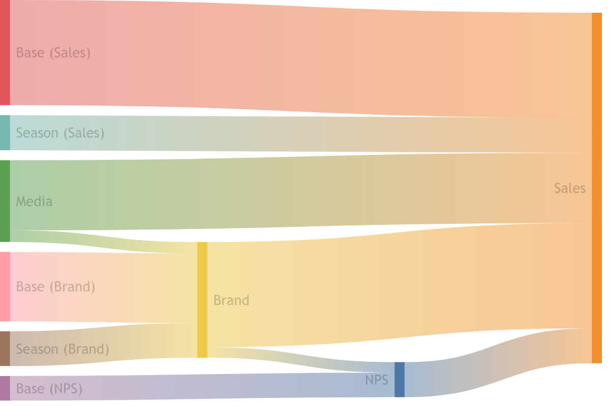
Total attribution is where the bookkeeping starts earning its keep. The method is the same as before: trace paths either backwards from the response or forwards from each leaf. The answer’s in Table 2.
| Variable | Direct connection | Indirect connection | Total |
|---|---|---|---|
| Base (Sales) | 30% | 0% | 30% |
| Season (Sales) | 10% | 0% | 10% |
| Base (Brand) | 0% | \(0.6 \times 0.3 + 0.6 \times 0.3 \times 0.1\) = 19.8% | 19.8% |
| Season (Brand) | 0% | \(0.3 \times 0.3 + 0.3 \times 0.3 \times 0.1\) = 9.9% | 9.9% |
| Base (NPS) | 0% | \(0.7 \times 0.1\) = 7% | 7% |
| Media | 20% | \(0.1 \times 0.3 + 0.1 \times 0.3 \times 0.1\) = 3.3% | 23.3% |
| Total | 70% | 30% | 100% |
Look at the Media row. Media has a direct path (20%), a path through Brand (Media -> Brand -> Sales = \(0.1 \times 0.3 = 3\%\)), and a path through Brand and then NPS (Media -> Brand -> NPS -> Sales = \(0.1 \times 0.3 \times 0.1 = 0.3\%\)). That’s 23.3% total. The same logic applies to every other leaf. You do the algebra once and then it’s just a walk along the graph.
Visually, I find the Sankey diagram in Figure 4 the easiest way to internalize what’s happening. You can see the volume of Sales flowing backwards, through the intermediate responses, and fanning out into the leaves.
Why this matters for how you report
The technical argument is neat. The practical consequence is where teams get burned.
If you report Total attribution for your leaf drivers and also report that “Brand contributes 30% to Sales”, you have double-counted. Brand’s contribution has already been decomposed and handed out to Base (Brand), Season (Brand), and Media. Reporting it again, on top of those, makes your numbers sum to something greater than 100%, and makes it look like your marketing is doing more than it is. I’ve seen this in real decks. It’s not a rounding error. It’s a category mistake.
The principled way to report results in a hierarchical MMM is to pick your lens deliberately:
- For optimization decisions (where should the next euro go?), you almost always want Total attribution on leaf drivers. You’re asking about actionable levers, and Media or Base (Brand) are levers. Brand is not a lever you can buy directly.
- For diagnostic storytelling (what’s driving what?), Direct attribution gives you the immediate explanation. It tells you that Brand carries 30% of Sales in the most recent period, which is a useful thing to know when you’re trying to understand the shape of the business.
Just don’t mix them in the same table. Pick a lens. Label it clearly. Stick to it.
Where Alviss AI sits on this
We build hierarchical Bayesian MMMs at Alviss AI, and this is exactly the kind of thing we’ve had to get opinionated about. When you model a business holistically, with Brand, NPS, Customer Experience, or any other intermediate KPI as first-class responses, you inherit the attribution question in full. The platform enforces the distinction between Direct and Total attribution explicitly, and it won’t let you sum them into the same column. Not because we enjoy being strict, but because the arithmetic quietly breaks if you do.
The upside of modeling this way, of course, is that you get to ask richer questions. How much of my Media spend is earning its keep by building Brand rather than driving Sales this week? is a question that a flat MMM can’t answer at all. A hierarchical one can, cleanly, as long as you’re disciplined about which attribution lens you’re using when.
Conclusion
Attribution in a neural network based MMM isn’t one thing. It’s at least two things: Direct, which only counts edges one step from the response, and Total, which traces every path back to the leaves. Both are legitimate. Neither is wrong. But they answer different questions, and the moment you have intermediate responses in your model (Brand, NPS, anything you’ve chosen to explain rather than just consume), you have to commit to one.
The rule I’d leave you with: any response node in your graph contributes zero to the Total attribution of something downstream of it. If that feels counter-intuitive, go back to Table 1 and stare at it until it doesn’t. And if your current reporting has Brand and Media both contributing to Sales under the same definition, you have some bookkeeping to do.
If you want to talk about how this shows up in your own modeling setup, or you think I’ve missed something (which happens), reach out. I’d rather be corrected than comfortable.